Tibor Vámos – László Keviczky–Ruth Bars – Dávid Sik
Methodology of Teaching the First Control Course
System view, understanding systems and how they are controlled is an important discipline in engineering education. Systems are all around us. Basic knowledge about them is important for everybody. Engineers need deep knowledge enabling analysis and design of control systems. Nowadays considering the ever increasing knowledge, the explosion of information available at the internet, the available visual technics and software tools there is a need to revisit the content and the teaching methodology of the first control course.
Considering the software supporting the control courses basically we can observe three directions.
a) Developing programming knowledge and new high level tools for solving control problems.
b) Application of ready program modules and applications (Guzmán et al., 2006, 2014). Here the common platform (Java, C, Matlab, etc) and harmonizing of the different operation systems (Windows, Unix, OS X) should be ensured.
c) Exploratory style using MATLAB. We encourage and guide the students to solve control problems using basic knowledge in MATLAB.
In our experience we prefer method c./ for which we published lecture notes (Keviczky et al. 2019b) providing collection of well chosen exercises. Ready program modules (point b./) are also applied mainly for demonstration and visualization.
A basic control course held for software engineering students at the Budapest University of Technology and Economics in the spring semester, 2019 covered the topics of analysis and design of continuous and discrete control systems. The content of the course and the teaching methodology were overviewed to respond to the challenges of the new teaching environment. A new aspect in the content of the course is the introduction of the YOULA parameterized controller design, which is a very effective method. The other controller algorithms can be considered as special cases of YOULA parameterization.
Considering the teaching methodology we tried to explain the main disciplines in an understandable way to everybody and then going into the precise mathematical description. Some interactive demonstrations presented during the lectures could provide the joy of understanding. Active participation of the students was ensured by problem solving at the end of the lectures and by the computer laboratory exercises using software MATLAB/SIMULINK. The students can contribute to the teaching material by elaborating their own case studies about a system and its control.
Content of a first control course
The course discusses analysis and design of both continuous and discrete linear control systems. Nowadays discrete control systems gain increasing importance in computer control of industrial processes. It is shown how well elaborated methods for investigation of continuous control systems can be imported to the discrete environment. Real systems are generally nonlinear, which can be handled individually. For analysis of linear systems there are general methods. Therefore it is expedient to linearize the systems in a given environment and apply control methods using the linearized models of the systems. Input/output models and also state space models are used to describe the systems. The control system should ensure the required prescribed performance of the plant. The controller is designed considering the model of the plant and the quality specifications. Controller design methods are discussed both for input/output models and state space models.
8 lectures have been elaborated and are available in ppt form covering the following topics:
1. Lecture: Introduction. Systems and control everywhere. System and their models. Analysis methods of continuous time linear systems.
2. Lecture: Analysis in the frequency domain. Relations between the time, Laplace operator and frequency domain.
3. Lecture: Feedback control systems. Stability analysis. Quality specifications formulated in the time and in the frequency domain. Control structures improving disturbance rejection. PID controller design.
4. Lecture: State space representation.
5. Lecture: Controllability, observability, state feedback, state estimation.
6. Lecture: Sampled-data (discrete) control systems. Analysis in the time- and in the z-operator domain.
7. Lecture: Description of discrete systems in the frequency domain. Relation to the continuous frequency functions. Discrete PID controller design. Discrete state equations. State feedback, state estimation.
8. Lecture: Control of discrete systems with time delay. Youla parameterization. Smith predictor. Dead-beat control. Outlook.
The lectures are available in English and in Hungarian at web-site https://www.aut.bme.hu/Course/szabtech
Recently published Springer textbooks (Keviczky et al., 2019a, 2019b) support the learning process. We refer also to the textbook of Åström and Murray (2008) available on the internet.
About the methodology of teaching the first control course
In the 3 hours of the lectures 2 hours are devoted for lecturing and presentation, in the next hour the students solve problems and then get immediate feedback of the solutions. For good solutions they get extra points considered in the results of the tests. Besides, during the semester they have to fulfill a project designing continuous and discrete controller for a given plant.
Besides these lectures two problem solving lectures support the students in preparing for the tests. Every second week the students solve MATLAB/SIMULINK exercises with the guidance of the teacher.
In the learning process it is important to understand the basic concepts and analyze the behavior of the systems with appropriate methods in order to design their control.
Besides listening to the presentations visual interactive demonstrations have a convincing strength while providing also the joy of learning. Active problem solving using software MATLAB/SIMULINK means learning by doing, while hopefully the students get some expert knowledge in analysis and design of control systems.
Levels of understanding, sysbook platform, interactive demonstrations
Systems and control are all around us.
System view, understanding systems and how they are controlled is important for everyone. The behavior of systems and the basic ideas of their control are determined by some fundamental principles which can be understood by everyone. The idea of T. Vámos dating back for 20 years was to present the main principles governing systems and control on different levels, for everyone, for students, for control experts (Vámos et al., 1999, 2016, 2018, Benedek et al. 2019). Nowadays there is an ever increasing demand to explain these concepts to everyone, simply and especially for non-engineering students (Albertos and Mareels, 2010).
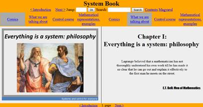
A multi-level e-book has been developed by T. Vámos and coworkers available at http://sysbook.sztaki.hu/.
The first level – knowledge for everyone (Fig. 1.) appears in cartoon like form with explanations.
.
Fig. 1. Ideas about systems can be explained for everyone
The second level gives deeper explanations with mathematical descriptions. Some animations and interactive (Java) files demonstrate the main concepts. During the lectures these parts of Sysbook are used for demonstration.
As examples Fig. 2 demonstrates that control of some systems can be a difficult task. A rod balanced by the juggler is an unstable plant, the so-called inverted pendulum. Taking a shower requires appropriate actions when changing the position of the taps considering the time delay of the process. Driving a car should avoid a number of disturbances when following the road and keeping the speed. Control is based on negative feedback, compares the measured output variable with its reference value, and uses the difference to modify the input variable of the system.
Fig. 2. Basic control idea: negative feedback. Control of difficult systems is a sophisticated task.
Analysis of systems in the time and in the frequency domain and their relationship is illustrated by an interactive demonstration shown in Fig. 3. It presents that taking more sinusoidal components in the periodic input signal the output of the system will be better approximated by the sum of the individual output components. So from the frequency response consequences can be made for the time response of a system.
Figure 4 shows an interactive file where the step response and the frequency response of a system can be shown. The parameters of the system can be changed and the responses are visualized.
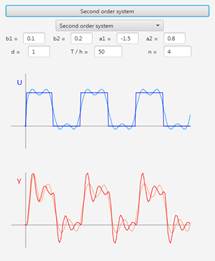
Fig. 3. Demonstration of the relationship between the time and the frequency domain
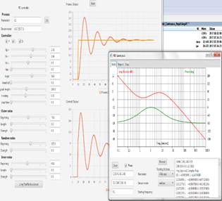
Fig. 4. Time and frequency responses of a system
Several control algorithms are discussed. Their behavior is demonstrated analyzing how the system tracks the reference signal, how it rejects the effect of the disturbances, how parameter uncertainties influence the performance, what is the effect of the filters. Figure 5 demonstrates the behavior of the YOULA parameterized controller.
We refer here also to the interactive tools developed by Guzmán et al. (2006, 2014) for PID controller design.
New paradigm in the basic control course: youla parameterization
As a new feature YOULA parameterization has been introduced as an essential control idea in the basic control course (Keviczky and Bányász, 2015). This approach follows in a straightforward way from the basic feedback control idea and provides good properties for the control system especially in case of big dead time. The introduction of this paradigm is shown in the sequel.
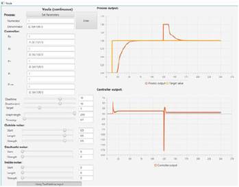
Fig. 5. Interactive file demonstrating the behavior of YOULA parameterized controller
In the theoretical part of the curriculum properties of negative feedback, the basic control principle are discussed. The block diagram of the control structure is shown on Fig. 6, where P is the model of the plant to be controlled, C is the algorithm of the controller and F is the input filter.
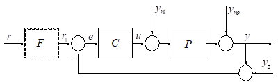
Fig. 6. Control is realized by negative feedback
This structure is effective ensuring reference signal tracking and disturbance rejection. The controller C is designed for the model of the plant considering the quality specifications. The most frequently applied algorithm is PID controller.
Supposing a unity filter F an equivalent structure between the output y and the input r is given on Fig. 7. Q is called the YOULA parameter. Reference signal tracking would be ideal if the Q controller would realize the inverse of the process model.
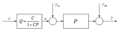
Fig. 7. Equivalent control structure with the YOULA parameter
This structure can not reject the effect of the disturbances. Therefore it is enhanced with Internal Model Control (IMC) (Garcia and Morari, 1982) according to Fig. 8.
YOULA parameterized control can be used to control stable processes.
Generally the inverse of the process can not be realized. The process model P should be separated to the invertible P+ part whose poles can be cancelled and to the non-invertible part ![]() which contains the dead time and the non-cancellable poles. The YOULA parameter realizes the inverse of the invertible part of the process model (Fig. 9.).
which contains the dead time and the non-cancellable poles. The YOULA parameter realizes the inverse of the invertible part of the process model (Fig. 9.).
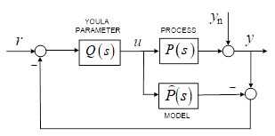
Fig. 8. YOULA parameterized control with IMC
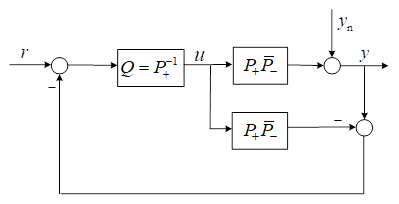
Fig. 9. Realizable YOULA parameterized control
This structure can be enhanced by the Rr reference and Rn disturbance filters according to Fig. 10.
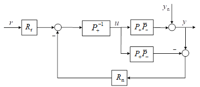
Fig. 10. YOULA parameterized control enhanced with filters
The role of the filters is threefold: the dynamics of reference signal tracking and disturbance rejection can be different, the maximum value of the control signal u can be restricted, and by appropriate choice of the filters the control system can be made more robust, i.e. more insensitive to model uncertainties.
This structure can be applied both for continuous and discrete systems. For discrete systems the pulse transfer function is denoted by G.
Figure 11 shows the output and control signals for control of a discrete second order system with big dead time when cancelling the whole dynamics. Oscillations in the control signal will cause intersampling oscillations in the output signal, while reaching the required reference value in the sampling points. Figure 12 gives the signals when only the invertible part is inverted in the controller. It is seen that the control performance became calm. Here filters were not applied.
It is shown that other control algorithms as PID, Smith predictor, dead-beat control can be considered as special cases of the YOULA parameterized algorithm.
The YOULA parameterized algorithm is especially effective when the process contains big dead time, and with appropriate design of the filters it is less sensitive to parameter uncertainties than the other algorithms.
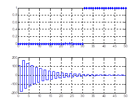
Fig. 11. Output and control signals when the YOULA parameter cancels the whole dynamics
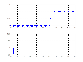
Fig. 12. Output and control signals when the YOULA parameter cancels only the invertible part of the model
Matlab/simulink computer exercises
The basic software applied in the computer laboratories is MATLAB/SIMULINK. The students get some expertise in applying analysis and synthesis methods in problem solving.
A MATLAB exercise description gives a short summary of the considered topic and then provides the examples from the simplest to the more complex ones. A MATLAB exercise related to a given topic can be executed within a two hour time frame and provides the knowledge for further individual work in the given topic. The students generally do not get a ready program, they have to build it command by command. This way they have to think over and understand the analysis or design procedure step by step. Based on these computer exercises every student has to be prepared to solve basic control problems and to solve his/her homework project. The MATLAB exercises cover the following topics: Introduction to MATLAB/SIMULINK and to the control toolbox. Properties and characteristics of typical control elements in the time and in the frequency domain. Stability analysis. PID controller design. State space description. Controllability, observability. State feedback, state estimation. Sampled data control systems. Z-transform and pulse transfer functions. Controller design based on the Youla parametrization. Discrete PID controller design. Smith predictor. Dead beat control. In some cases the problem is solved using MATLAB, then a SIMULINK program is built to simulate the behaviour of the control system. In some cases a core program is given for a specific problem and the student give the input data and running the program they evaluate the behaviour of the system.
As an example the core program of the discrete YOULA parameterization is presented in the sequel.
% Youla_discrete basic program
display('... Q='),Q=minreal(Rn/Gp,0.0001)
display('... C='),C=minreal(Q/(1-Q*G),0.0001)
display('... L='),L=minreal(C*G,0.0001)
display('...Tr='),Tr=minreal((Rr/Rn)*Q*G,0.0001)
display('..Ur='),Ur=minreal((Rr/Rn)*Q,0.0001)
pause
t=0:Ts:50;
figure(1)
yr=step(Tr,t);
subplot(211), plot(t,yr,'*'),grid
ur=step(Ur,t);
subplot(212), stairs(t,ur),grid
pause;
display('.....Sn='),Sn=minreal((1-Q*G),0.0001)
display('.....Un='),Un=minreal(-C*(1-Q*G,0.0001)
pause
figure(2)
yn=step(Sn,t);
subplot(211),plot(t,yn,'*'),grid;
un=step(Un,t);
subplot(212),stairs(t,un),grid;
Then give the second order process, the sampling time, its separation and the filters in MATLAB,
clear; clc; s=zpk('s')
P=1/((1+5*s)*(1+10*s))
Ts=1; z=zpk('z',Ts); G1=c2d(P,Ts)
G=G1*z^(-30)
Gm=1; %G-
Gp=G1/Gm %G+
Rr=1/z; Rn=1/z;
and call the program. The behaviour of the algorithm can be investigated with different separation and with different filters. The SIMULINK diagram can be built enabling analysis of intersampling behaviour as well.
The MATLAB exercises are given in Keviczky et al. (2019b).
Open content development - student case studies
Nowadays in education a new teaching – learning paradigm is Open Content Development (OCD) which means active participation of the teachers and students creating an up-to-date teaching material. This project runs at the Department of Technical Education at the Budapest University of Technology and Economics since 2015 supported by the Hungarian Academy of Sciences. In the frame of vocational teacher training programs several so-called micro-contents have been developed. Utilizing the experiences of these pilot efforts this approach seemed to be fruitful also in basic control education.
The Sysbook platform has been connected to the OCD model. In a special surface Sysbook provides several case studies for systems and their control (e.g. driving, energy production and distribution, oil refinery, systems and control in the living organism, etc.). Teachers and students studying systems and control can elaborate new case studies in their areas of interest which means active application of the learned topics. After evaluation these projects can be uploaded in the student area of Sysbook.
The system chosen by the learner for analysis is modelled and its control aspects are also considered. In the different examples it is investigated, what is considered a system, how is the system connected to its environment, what are the input signals and what are the output signals? What happens between them? How can this be described mathematically? What are the requirements set for the system? Which balance and energy considerations have to be applied? Can we control the system? How to control the system?
Till now some uploaded student projects are temperature control of a terrarium, speed control, model of the blood circulation and the respiratory system, the model of building a house, organising sport activity in the school, etc. (Fig. 13.)
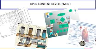
Fig. 13. Some student projects
Later on the student’s will be able to rate and comment on each other contribution to the Sysbook. The evaluation of the students can be made with the Sysbook’s cooperation with a Moodle based course. This evaluation environment gives some very useful tools for creating and evaluating questionnaire: automatic timer control, different types of questions and feedback about the results.
The system open for the participating students/learners and educators is accessible through the research web page (www.ocd.bme.hu); the page also contains Bring Your Own Device (BYOD) approaches that serve the methodological support of the innovations implemented within the open system.
Conclusion
In the methodology of teaching a basic control course the motivation of the students can be increased by active participation in the learning process, including interactive demonstration of the principles, solving exercises at the end of the lectures and getting immediate feedback, solving analysis and synthesis problems in the computer laboratories, and developing their own case studies for Sysbook in OCD framework.
It should be also emphasized that the examples of systems and their control should be chosen mainly from the area of the specialization of the students (electrical or software engineering, chemical engineering, biology, economics, etc. (A. Leva, 2016)). Also it is important to provide real-time experiments in laboratory work or using distant laboratories. IFAC Repository would be also of great help reaching useful resources.
REFERENCES
· Albertos, P., Mareels, I. (2010). Feedback and Control for Everyone. Springer.
· Åström, K. J., Murray, R.M. (2008). Feedback Systems: An Introduction for Scientists and Engineers.
· Princeton University Press, http://www.cds.caltech.edu/~murray/books/AM05/pdf/am08-complete_22Feb09.pdf
· Benedek A., Vámos T., Bars R., Sik D. (2019). Open Content Development Applied in Learning Systems and Control, European Control Conference (ECC). Nápoly, Italy. pp. 3059-3064.
· Garcia, C.E., Morari, M.: Internal Model Control 1. A Unifying Review and Some New Results (1982). Industrial & Engineering Chemistry Process Design and Development, 21 (2): 308–323.
· Guzmán, J. Luis, Hägglund, T., Åström, K. J., Dormido, S., Berenguel, M. and Piquet, Y. (2014). Understanding PID design through interactive tools. 19th IFAC World Congress, Cape Town.
· Guzmán, J. Luis, Åström, K. J., Dormido, S., Hägglund, T., Piquet, Y. (2006). Interactive Learning Modules for PID Control. IFAC Proceedings Volumes 39(6): 7-12.
· Keviczky, L., Bars, R., Hetthéssy, J., Bányász, Cs. (2019a). Control Engineering. Springer.
· Keviczky, L., Bars, R., Hetthéssy, J., Bányász, Cs. (2019b). Control Engineering: MATLAB Exercises. Springer.
· Keviczky, L., Bányász, Cs. (2015). Two-Degree-of-Freedom Control Systems, The Youla Parameterization Approach, Academic Press, Elsevier.
· Leva, A. (2018). Teaching PID control to computer engineers: a step to fill a cultural gap (2018). 11th IFAC Symp. on Advances in Control Education, ACE’2016, Bratislava, Slovakia, IFAC-PapersOnline Vol. 51, Issue 4, pp. 328-333.
· Vámos, T., Bokor J. and Hangos, K. (1999). Systems - governing principles and multimedia /CD/. 14th IFAC World Congress, Beijing, China, PT-5, p. 79. Plenary lecture.
· Vámos, T., Bars, R. and Sik, D. (2016). Bird’s Eye View on Systems and Control – General View and Case Studies. 11th IFAC Symp. on Advances in Control Education, ACE’2016, Bratislava, Slovakia, IFAC-PapersOnline Vol. 49, Issue 6, pp. 274-279.
· Vámos, T., Keviczky, L., Bars, R., Benedek, A., Sik D. (2018). An Introductory Overview About Systems and Control: A Motivation Lecture in Control Education. 26th Mediterranean Conference on Control and Automation (MED’2018). Zadar, Croatia.